
Size each GPU correctly
Separate expert weights, replicated layers and attention state. Use pinned configurations to see why Qwen, Kimi and gpt-oss need different cache calculations.
Handbook 03 / September 2026
DeepSeek, Qwen, Kimi, GLM and gpt-oss in production
Turn a promising model into a service you can size and operate. Follow one private coding assistant through model selection, per-GPU memory, expert communication, engine validation, recovery and cost. Work through three design rounds with complete answers.
PDF and Python companion included with Premium. Keep the copies you download.
Already a member? Sign in to download →
Separate expert weights, replicated layers and attention state. Use pinned configurations to see why Qwen, Kimi and gpt-oss need different cache calculations.
Check formats, tool loops, precision and speculation before measuring the load curve. Learn which evidence belongs in a release record.
Set context limits, account for lost replicas and interrupted streams, then compare cost using accepted work over the full billing period.
Inside the guide
Explore the sample pages →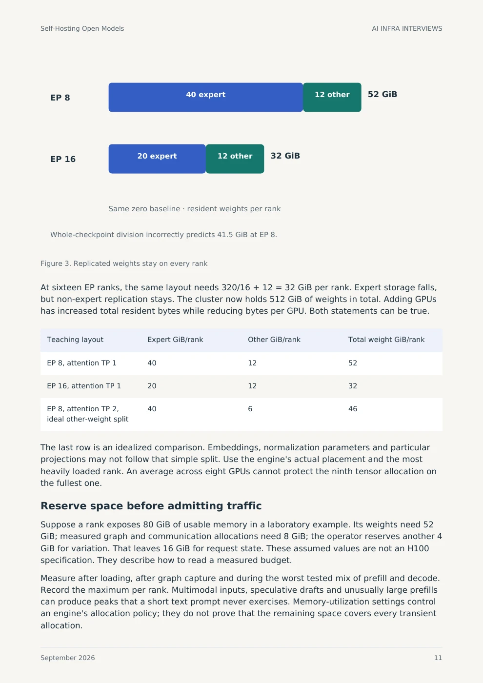
These are complete selected pages, with text versions of their diagrams and tables.
Figure 3. Replicated weights stay on every rank
At sixteen EP ranks, the same layout needs 320/16 + 12 = 32 GiB per rank. Expert storage falls, but non-expert replication stays. The cluster now holds 512 GiB of weights in total. Adding GPUs has increased total resident bytes while reducing bytes per GPU. Both statements can be true.
| Teaching layout | Expert GiB/rank | Other GiB/rank | Total weight GiB/rank |
|---|---|---|---|
| EP 8, attention TP 1 | 40 | 12 | 52 |
| EP 16, attention TP 1 | 20 | 12 | 32 |
| EP 8, attention TP 2, ideal other-weight split | 40 | 6 | 46 |
The last row is an idealized comparison. Embeddings, normalization parameters and particular projections may not follow that simple split. Use the engine's actual placement and the most heavily loaded rank. An average across eight GPUs cannot protect the ninth tensor allocation on the fullest one.
Suppose a rank exposes 80 GiB of usable memory in a laboratory example. Its weights need 52 GiB; measured graph and communication allocations need 8 GiB; the operator reserves another 4 GiB for variation. That leaves 16 GiB for request state. These assumed values are not an H100 specification. They describe how to read a measured budget.
Measure after loading, after graph capture and during the worst tested mix of prefill and decode. Record the maximum per rank. Multimodal inputs, speculative drafts and unusually large prefills can produce peaks that a short text prompt never exercises. Memory-utilization settings control an engine's allocation policy; they do not prove that the remaining space covers every transient allocation.
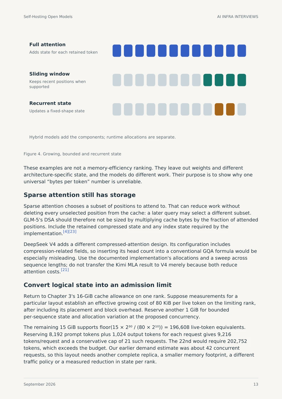
Figure 4. Growing, bounded and recurrent state
These examples are not a memory-efficiency ranking. They leave out weights and different architecture-specific state, and the models do different work. Their purpose is to show why one universal “bytes per token” number is unreliable.
Sparse attention chooses a subset of positions to attend to. That can reduce work without deleting every unselected position from the cache: a later query may select a different subset. GLM-5's DSA should therefore not be sized by multiplying cache bytes by the fraction of attended positions. Include the retained compressed state and any index state required by the implementation.[4][23]
DeepSeek V4 adds a different compressed-attention design. Its configuration includes compression-related fields, so inserting its head count into a conventional GQA formula would be especially misleading. Use the documented implementation's allocations and a sweep across sequence lengths; do not transfer the Kimi MLA result to V4 merely because both reduce attention costs.[21]
Return to Chapter 3's 16-GiB cache allowance on one rank. Suppose measurements for a particular layout establish an effective growing cost of 80 KiB per live token on the limiting rank, after including its placement and block overhead. Reserve another 1 GiB for bounded per-sequence state and allocation variation at the proposed concurrency.
The remaining 15 GiB supports floor(15 × 2³⁰ / (80 × 2¹⁰)) = 196,608 live-token equivalents. Reserving 8,192 prompt tokens plus 1,024 output tokens for each request gives 9,216 tokens/request and a conservative cap of 21 such requests. The 22nd would require 202,752 tokens, which exceeds the budget. Our earlier demand estimate was about 42 concurrent requests, so this layout needs another complete replica, a smaller memory footprint, a different traffic policy or a measured reduction in state per rank.
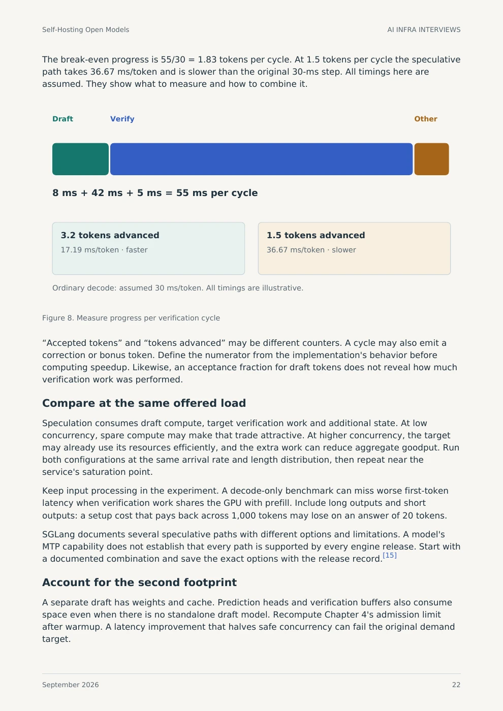
The break-even progress is 55/30 = 1.83 tokens per cycle. At 1.5 tokens per cycle the speculative path takes 36.67 ms/token and is slower than the original 30-ms step. All timings here are assumed. They show what to measure and how to combine it.
Figure 8. Measure progress per verification cycle
“Accepted tokens” and “tokens advanced” may be different counters. A cycle may also emit a correction or bonus token. Define the numerator from the implementation's behavior before computing speedup. Likewise, an acceptance fraction for draft tokens does not reveal how much verification work was performed.
Speculation consumes draft compute, target verification work and additional state. At low concurrency, spare compute may make that trade attractive. At higher concurrency, the target may already use its resources efficiently, and the extra work can reduce aggregate goodput. Run both configurations at the same arrival rate and length distribution, then repeat near the service's saturation point.
Keep input processing in the experiment. A decode-only benchmark can miss worse first-token latency when verification work shares the GPU with prefill. Include long outputs and short outputs: a setup cost that pays back across 1,000 tokens may lose on an answer of 20 tokens.
SGLang documents several speculative paths with different options and limitations. A model's MTP capability does not establish that every path is supported by every engine release. Start with a documented combination and save the exact options with the release record.[15]
A separate draft has weights and cache. Prediction heads and verification buffers also consume space even when there is no standalone draft model. Recompute Chapter 4's admission limit after warmup. A latency improvement that halves safe concurrency can fail the original demand target.
The downloadable Python companion runs on a CPU with the standard library. It reproduces the worked calculations and exercises the book’s simulated control paths. Its README explains the inputs and limits.
These are teaching calculations and fixtures. GPU serving, training and performance benchmarks were not run for this edition. Primary sources and dated configurations support the factual claims; each worked scenario states its assumptions.
Browse all illustrated guides →
LLM Inference Systems Design explains serving fundamentals. Distributed Inference on Kubernetes follows the workload across a cluster.