
Size the whole learning loop
Count training state, rollout cache and environment workers. Compare colocated and separate fleets using wall time, GPU time and eligible attempts.
Handbook 04 / September 2026
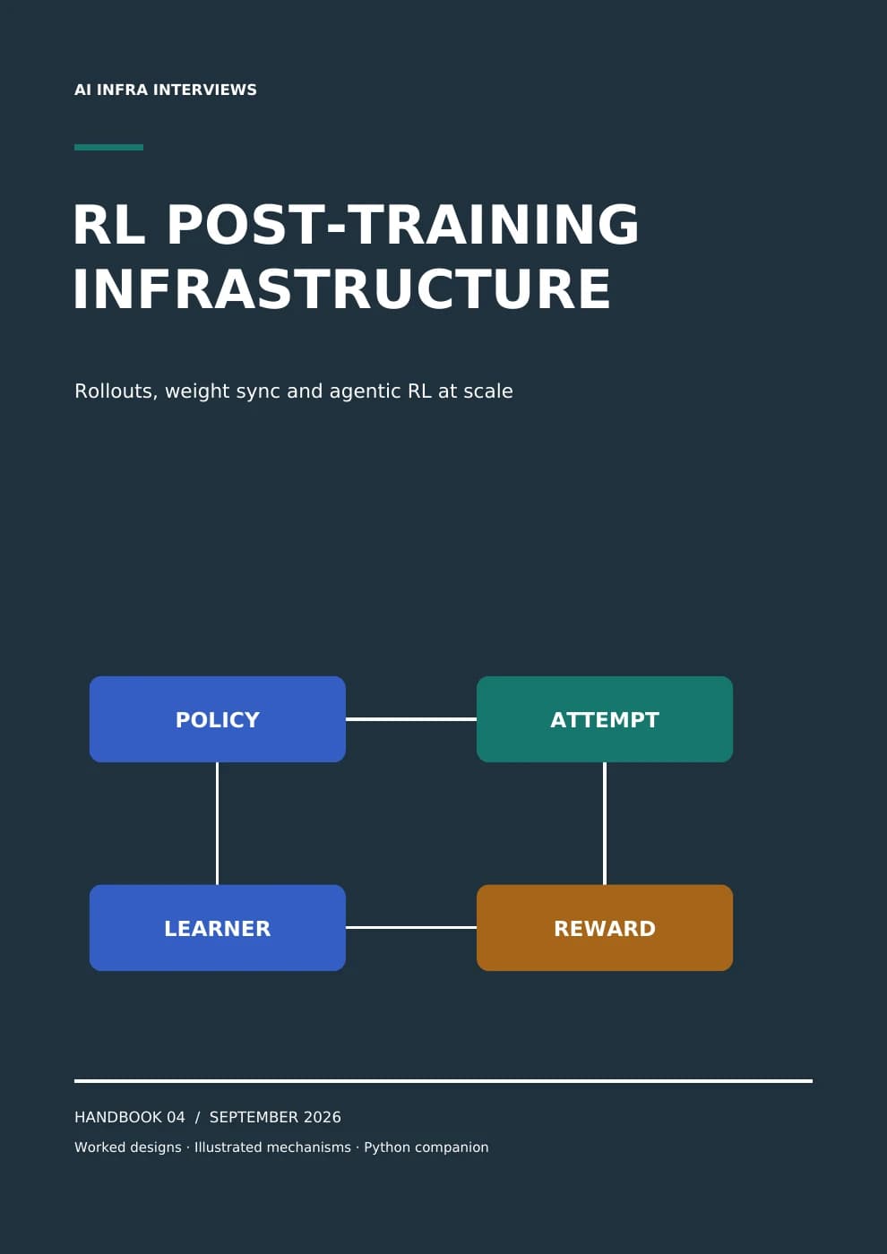
Rollouts, weight sync and agentic RL at scale
Follow a coding agent’s training run from its first attempt to a new policy. Size the actor and rollout fleet, publish weights safely, handle slow episodes and verify that the learner is training on the right tokens. Work through three complete design rounds.
PDF and Python companion included with Premium. Keep the copies you download.
Already a member? Sign in to download →
Count training state, rollout cache and environment workers. Compare colocated and separate fleets using wall time, GPU time and eligible attempts.
Trace staged policy updates, group completion and stale data. Understand probability corrections and the limits of numerical and routing replay checks.
Build a reproducible acceptance path, inspect held-out quality and restore a consistent checkpoint. Compare documented paths in verl, slime, OpenRLHF, NeMo RL and vime.
Inside the guide
Explore the sample pages →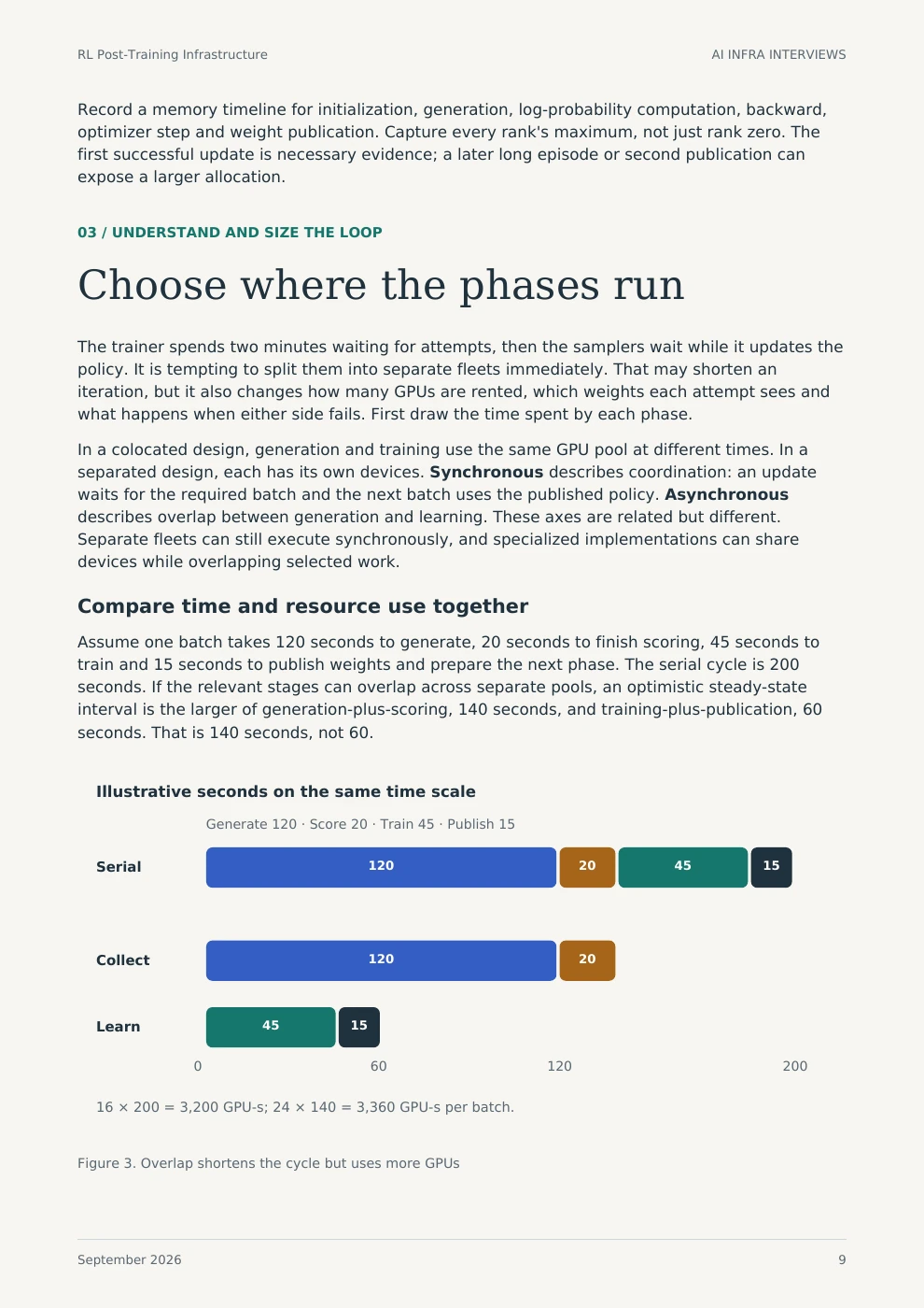
These are complete selected pages, with text versions of their diagrams and tables.
Record a memory timeline for initialization, generation, log-probability computation, backward, optimizer step and weight publication. Capture every rank's maximum, not just rank zero. The first successful update is necessary evidence; a later long episode or second publication can expose a larger allocation.
03 / UNDERSTAND AND SIZE THE LOOP
The trainer spends two minutes waiting for attempts, then the samplers wait while it updates the policy. It is tempting to split them into separate fleets immediately. That may shorten an iteration, but it also changes how many GPUs are rented, which weights each attempt sees and what happens when either side fails. First draw the time spent by each phase.
In a colocated design, generation and training use the same GPU pool at different times. In a separated design, each has its own devices. Synchronous describes coordination: an update waits for the required batch and the next batch uses the published policy. Asynchronous describes overlap between generation and learning. These axes are related but different. Separate fleets can still execute synchronously, and specialized implementations can share devices while overlapping selected work.
Assume one batch takes 120 seconds to generate, 20 seconds to finish scoring, 45 seconds to train and 15 seconds to publish weights and prepare the next phase. The serial cycle is 200 seconds. If the relevant stages can overlap across separate pools, an optimistic steady-state interval is the larger of generation-plus-scoring, 140 seconds, and training-plus-publication, 60 seconds. That is 140 seconds, not 60.
Figure 3. Overlap shortens the cycle but uses more GPUs
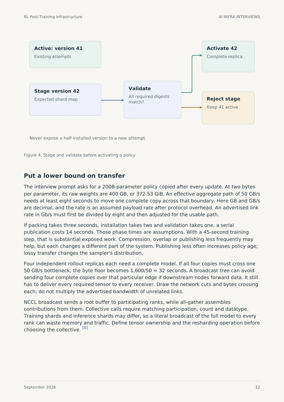
Figure 4. Stage and validate before activating a policy
The interview prompt asks for a 200B-parameter policy copied after every update. At two bytes per parameter, its raw weights are 400 GB, or 372.53 GiB. An effective aggregate path of 50 GB/s needs at least eight seconds to move one complete copy across that boundary. Here GB and GB/s are decimal, and the rate is an assumed payload rate after protocol overhead. An advertised link rate in Gb/s must first be divided by eight and then adjusted for the usable path.
If packing takes three seconds, installation takes two and validation takes one, a serial publication costs 14 seconds. Those phase times are assumptions. With a 45-second training step, that is substantial exposed work. Compression, overlap or publishing less frequently may help, but each changes a different part of the system. Publishing less often increases policy age; lossy transfer changes the sampler's distribution.
Four independent rollout replicas each need a complete model. If all four copies must cross one 50 GB/s bottleneck, the byte floor becomes 1,600/50 = 32 seconds. A broadcast tree can avoid sending four complete copies over that particular edge if downstream nodes forward data. It still has to deliver every required tensor to every receiver. Draw the network cuts and bytes crossing each; do not multiply the advertised bandwidth of unrelated links.
NCCL broadcast sends a root buffer to participating ranks, while all-gather assembles contributions from them. Collective calls require matching participation, count and datatype. Training shards and inference shards may differ, so a literal broadcast of the full model to every rank can waste memory and traffic. Define tensor ownership and the resharding operation before choosing the collective. [6]
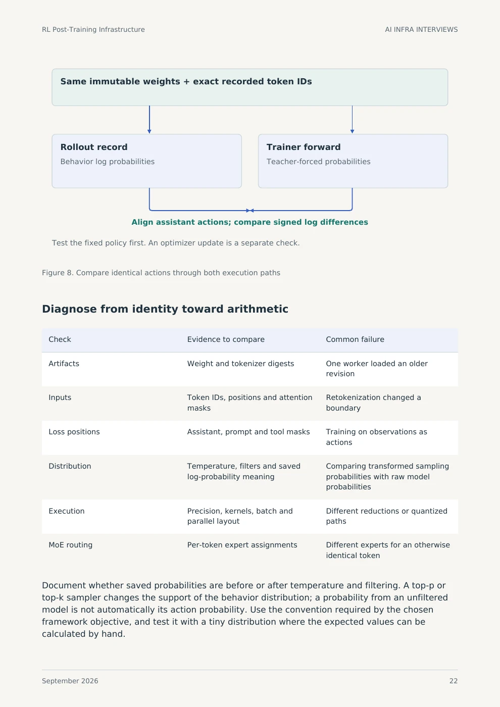
Figure 8. Compare identical actions through both execution paths
| Check | Evidence to compare | Common failure |
|---|---|---|
| Artifacts | Weight and tokenizer digests | One worker loaded an older revision |
| Inputs | Token IDs, positions and attention masks | Retokenization changed a boundary |
| Loss positions | Assistant, prompt and tool masks | Training on observations as actions |
| Distribution | Temperature, filters and saved log-probability meaning | Comparing transformed sampling probabilities with raw model probabilities |
| Execution | Precision, kernels, batch and parallel layout | Different reductions or quantized paths |
| MoE routing | Per-token expert assignments | Different experts for an otherwise identical token |
Document whether saved probabilities are before or after temperature and filtering. A top-p or top-k sampler changes the support of the behavior distribution; a probability from an unfiltered model is not automatically its action probability. Use the convention required by the chosen framework objective, and test it with a tiny distribution where the expected values can be calculated by hand.
The downloadable Python companion runs on a CPU with the standard library. It reproduces the worked calculations and exercises the book’s simulated control paths. Its README explains the inputs and limits.
These are teaching calculations and fixtures. GPU serving, training and performance benchmarks were not run for this edition. Primary sources and dated configurations support the factual claims; each worked scenario states its assumptions.
Browse all illustrated guides →
LLM Inference Systems Design explains serving fundamentals. Distributed Inference on Kubernetes follows the workload across a cluster.