
Explain the cost of a useful outcome
Separate tasks, attempts and tokens. Include tools, retries and human review, then build low, base and high demand budgets with explicit assumptions.
Handbook 05 / September 2026
Inference economics and capacity planning
Build an AI budget you can explain. Follow a useful customer task through model calls, retries, human review and the monthly bill. Work through API pricing, GPU capacity, caching, break-even and purchasing decisions, with seven free calculators and complete business scenarios.
PDF and Python companion included with Premium. Keep the copies you download.
Already a member? Sign in to download →
Separate tasks, attempts and tokens. Include tools, retries and human review, then build low, base and high demand budgets with explicit assumptions.
Read a load test, size whole replicas for peaks and failures, and see why a performance improvement may remove one deployment or none.
Compare API and fleet costs, rental and ownership, and the effect of commitments. Reconcile the bill and record the evidence that would change your choice.
Build an API budget, size peak capacity, compare API and fleet costs, or work through caching, routing and ownership. Each calculator shows its assumptions and formula, with a scenario you can save.
Open the economics workbench →No account needed. The starting numbers are hypothetical; replace them with your rates and measurements.
Inside the guide
Explore the sample pages →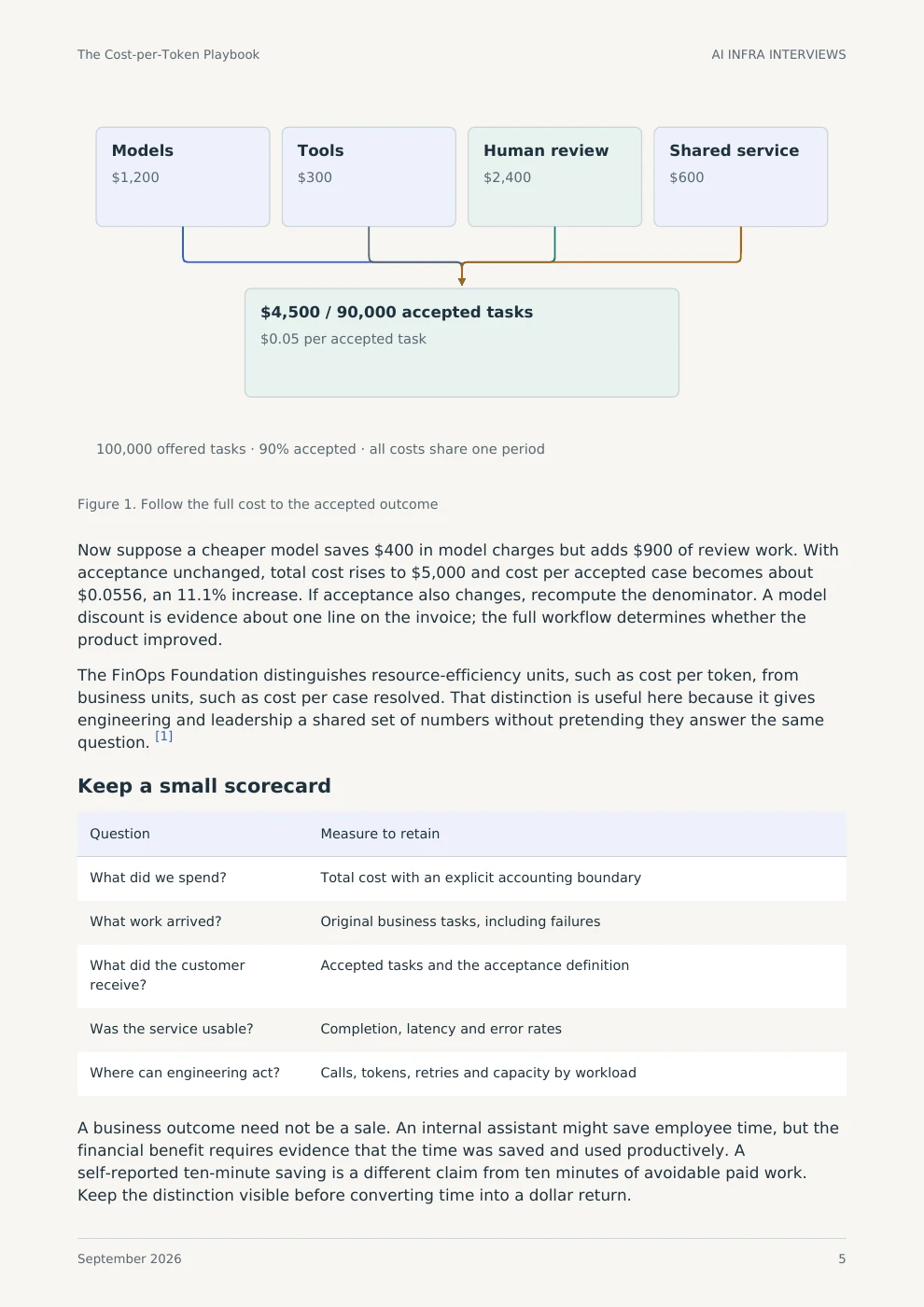
These are complete selected pages, with text versions of their diagrams and tables.
Figure 1. Follow the full cost to the accepted outcome
Now suppose a cheaper model saves $400 in model charges but adds $900 of review work. With acceptance unchanged, total cost rises to $5,000 and cost per accepted case becomes about $0.0556, an 11.1% increase. If acceptance also changes, recompute the denominator. A model discount is evidence about one line on the invoice; the full workflow determines whether the product improved.
The FinOps Foundation distinguishes resource-efficiency units, such as cost per token, from business units, such as cost per case resolved. That distinction is useful here because it gives engineering and leadership a shared set of numbers without pretending they answer the same question. [1]
| Question | Measure to retain |
|---|---|
| What did we spend? | Total cost with an explicit accounting boundary |
| What work arrived? | Original business tasks, including failures |
| What did the customer receive? | Accepted tasks and the acceptance definition |
| Was the service usable? | Completion, latency and error rates |
| Where can engineering act? | Calls, tokens, retries and capacity by workload |
A business outcome need not be a sale. An internal assistant might save employee time, but the financial benefit requires evidence that the time was saved and used productively. A self-reported ten-minute saving is a different claim from ten minutes of avoidable paid work. Keep the distinction visible before converting time into a dollar return.
08 / CONNECT THE BUDGET TO CAPACITY
A million requests per month sounds large until you divide it by time. Over a 30-day month, it averages about 0.386 requests/s. If most arrivals happen during a short daily window, the required serving rate can be many times higher. A monthly volume forecast pays for work; a peak forecast decides how much capacity must be ready at once.
State the interval behind “peak.” A five-minute average smooths bursts that may still overwhelm a two-second response target. Use arrival traces at the timescale that matters to the product, including launches, business hours and synchronized background jobs. Seasonal forecasts should identify which pattern is observed and which is a planning assumption.
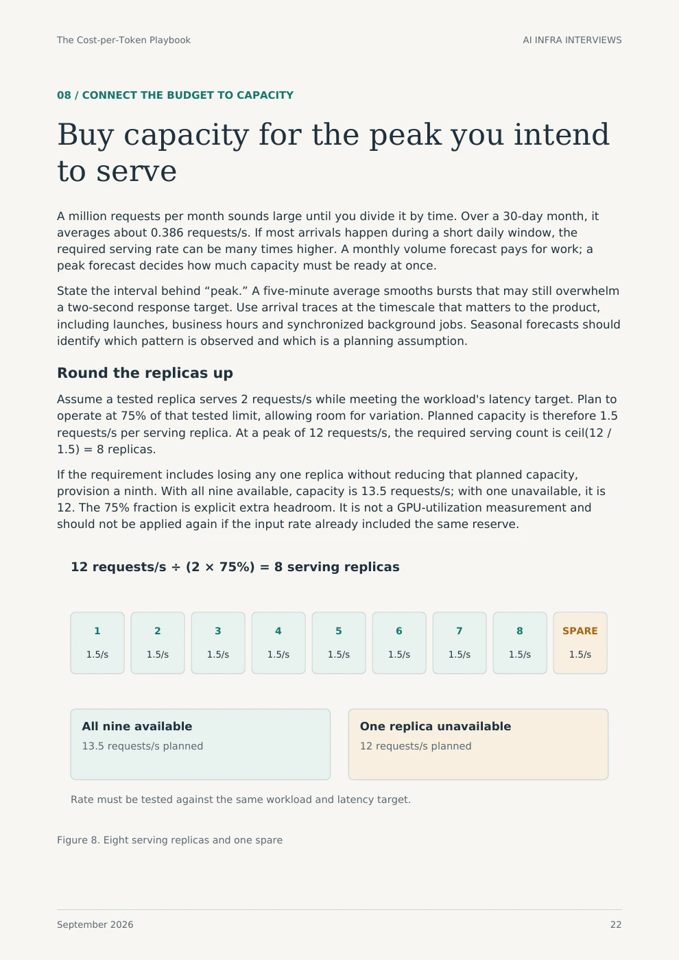
Assume a tested replica serves 2 requests/s while meeting the workload's latency target. Plan to operate at 75% of that tested limit, allowing room for variation. Planned capacity is therefore 1.5 requests/s per serving replica. At a peak of 12 requests/s, the required serving count is ceil(12 / 1.5) = 8 replicas.
If the requirement includes losing any one replica without reducing that planned capacity, provision a ninth. With all nine available, capacity is 13.5 requests/s; with one unavailable, it is 12. The 75% fraction is explicit extra headroom. It is not a GPU-utilization measurement and should not be applied again if the input rate already included the same reserve.
Figure 8. Eight serving replicas and one spare
10 / CONNECT THE BUDGET TO CAPACITY
A team presents a neat graph: two lines cross, so self-hosting becomes cheaper above that volume. The arithmetic may be correct within the fleet's current capacity. The missing question is what happens when the next request requires another deployment.
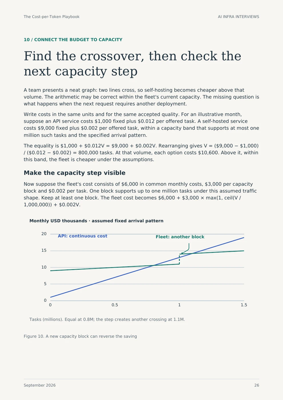
Write costs in the same units and for the same accepted quality. For an illustrative month, suppose an API service costs $1,000 fixed plus $0.012 per offered task. A self-hosted service costs $9,000 fixed plus $0.002 per offered task, within a capacity band that supports at most one million such tasks and the specified arrival pattern.
The equality is $1,000 + $0.012V = $9,000 + $0.002V. Rearranging gives V = ($9,000 − $1,000) / ($0.012 − $0.002) = 800,000 tasks. At that volume, each option costs $10,600. Above it, within this band, the fleet is cheaper under the assumptions.
Now suppose the fleet's cost consists of $6,000 in common monthly costs, $3,000 per capacity block and $0.002 per task. One block supports up to one million tasks under this assumed traffic shape. Keep at least one block. The fleet cost becomes $6,000 + $3,000 × max(1, ceil(V / 1,000,000)) + $0.002V.
Figure 10. A new capacity block can reverse the saving
The downloadable Python companion runs on a CPU with the standard library. It checks all seven calculator defaults and the book’s worked scenarios, including cache reuse, capacity steps, migration payback and discounted cash flow. Export your web scenario and rerun it offline. Its README explains the inputs and limits.
These are teaching calculations and fixtures. GPU serving, training and performance benchmarks were not run for this edition. Primary sources and dated configurations support the factual claims; each worked scenario states its assumptions.
Browse all illustrated guides →
LLM Inference Systems Design explains serving fundamentals. Distributed Inference on Kubernetes follows the workload across a cluster.