
Connect the estimate to the service
Distinguish a hardware ceiling from a memory bound and a measured rate. Read a load curve, name the failure domain, and allocate whole replicas against a stated contract.
Handbook 06 / September 2026
From the first estimate to a design you can defend
Build an architecture you can explain from the first estimate through a failed machine. Work through streaming inference, distributed training, shared GPU fleets and the systems around them. Follow the state, calculate the bottleneck, and test the decision with a harder workload.
Premium guide PDFs and companion files require an active paid Premium membership or approved complimentary access. Referral Premium includes the rest of the site, but excludes these downloads. Keep the copies you download.
Already a member? Sign in to download →

Distinguish a hardware ceiling from a memory bound and a measured rate. Read a load curve, name the failure domain, and allocate whole replicas against a stated contract.
Follow a KV handoff, a checkpoint commit, a resource lease and a usage reservation. Decide which acknowledgements are safe and what recovery can actually restore.
Rehearse three original design studios with worked answers and follow-up variations. Challenge an unsafe architecture, then state the evidence that would change your recommendation.
Inside the guide
Explore the sample pages →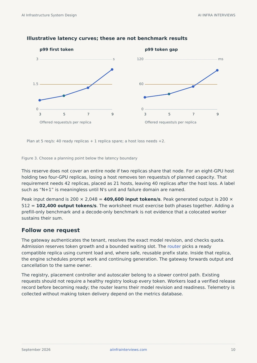
These are complete selected pages, with text versions of their diagrams and tables.
Figure 3. Choose a planning point below the latency boundary
This reserve does not cover an entire node if two replicas share that node. For an eight-GPU host holding two four-GPU replicas, losing a host removes ten requests/s of planned capacity. That requirement needs 42 replicas, placed as 21 hosts, leaving 40 replicas after the host loss. A label such as “N+1” is meaningless until N's unit and failure domain are named.
Peak input demand is 200 × 2,048 = 409,600 input tokens/s. Peak generated output is 200 × 512 = 102,400 output tokens/s. The worksheet must exercise both phases together. Adding a prefill-only benchmark and a decode-only benchmark is not evidence that a colocated worker sustains their sum.
The gateway authenticates the tenant, resolves the exact model revision, and checks quota. Admission reserves token growth and a bounded waiting slot. The router picks a ready compatible replica using current load and, where safe, reusable prefix state. Inside that replica, the engine schedules prompt work and continuing generation. The gateway forwards output and cancellation to the same owner.
The registry, placement controller and autoscaler belong to a slower control path. Existing requests should not require a healthy registry lookup every token. Workers load a verified release record before becoming ready; the router learns their model revision and readiness. Telemetry is collected without making token delivery depend on the metrics database.
PyTorch's asynchronous checkpoint recipe explains the staging memory cost and recommends controlling outstanding checkpoint work. Async saving moves work off the training path; it does not remove the memory or storage work. [13]
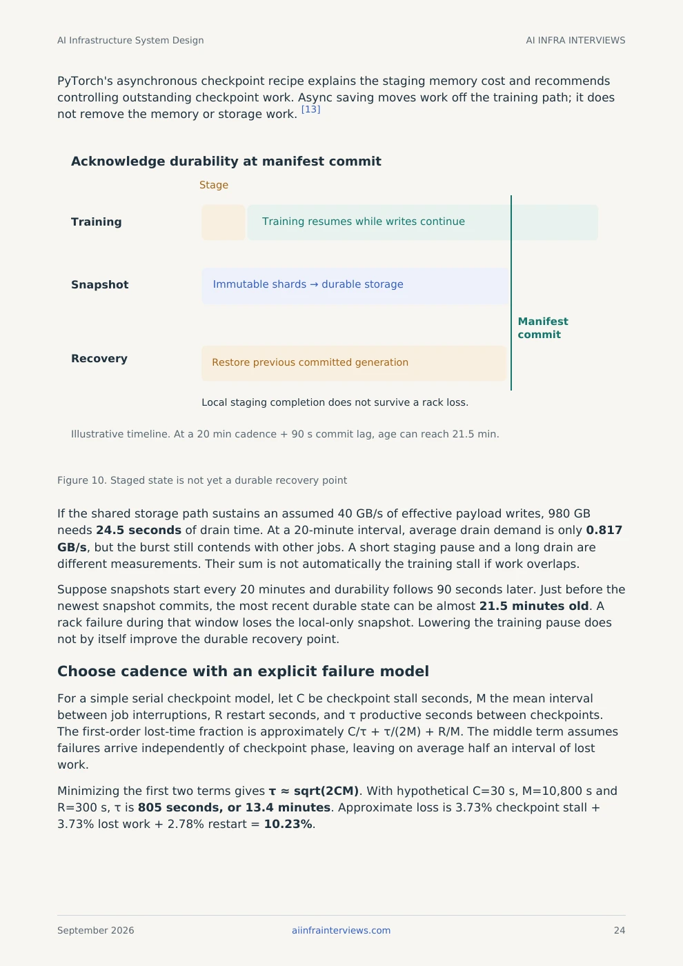
Figure 10. Staged state is not yet a durable recovery point
If the shared storage path sustains an assumed 40 GB/s of effective payload writes, 980 GB needs 24.5 seconds of drain time. At a 20-minute interval, average drain demand is only 0.817 GB/s, but the burst still contends with other jobs. A short staging pause and a long drain are different measurements. Their sum is not automatically the training stall if work overlaps.
Suppose snapshots start every 20 minutes and durability follows 90 seconds later. Just before the newest snapshot commits, the most recent durable state can be almost 21.5 minutes old. A rack failure during that window loses the local-only snapshot. Lowering the training pause does not by itself improve the durable recovery point.
For a simple serial checkpoint model, let C be checkpoint stall seconds, M the mean interval between job interruptions, R restart seconds, and τ productive seconds between checkpoints. The first-order lost-time fraction is approximately C/τ + τ/(2M) + R/M. The middle term assumes failures arrive independently of checkpoint phase, leaving on average half an interval of lost work.
Minimizing the first two terms gives τ ≈ sqrt(2CM). With hypothetical C=30 s, M=10,800 s and R=300 s, τ is 805 seconds, or 13.4 minutes. Approximate loss is 3.73% checkpoint stall + 3.73% lost work + 2.78% restart = 10.23%.
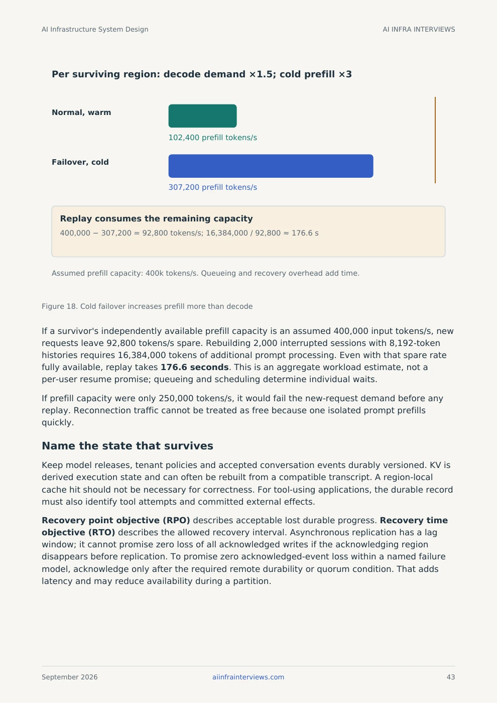
Figure 18. Cold failover increases prefill more than decode
If a survivor's independently available prefill capacity is an assumed 400,000 input tokens/s, new requests leave 92,800 tokens/s spare. Rebuilding 2,000 interrupted sessions with 8,192-token histories requires 16,384,000 tokens of additional prompt processing. Even with that spare rate fully available, replay takes 176.6 seconds. This is an aggregate workload estimate, not a per-user resume promise; queueing and scheduling determine individual waits.
If prefill capacity were only 250,000 tokens/s, it would fail the new-request demand before any replay. Reconnection traffic cannot be treated as free because one isolated prompt prefills quickly.
Keep model releases, tenant policies and accepted conversation events durably versioned. KV is derived execution state and can often be rebuilt from a compatible transcript. A region-local cache hit should not be necessary for correctness. For tool-using applications, the durable record must also identify tool attempts and committed external effects.
Recovery point objective (RPO) describes acceptable lost durable progress. Recovery time objective (RTO) describes the allowed recovery interval. Asynchronous replication has a lag window; it cannot promise zero loss of all acknowledged writes if the acknowledging region disappears before replication. To promise zero acknowledged-event loss within a named failure model, acknowledge only after the required remote durability or quorum condition. That adds latency and may reduce availability during a partition.
The downloadable Python companion runs on a CPU with the standard library. Run the book’s arithmetic on a CPU: model memory, replica capacity, KV transfers, training time, checkpoint cadence, evaluation demand and regional recovery. Change an input in the scenario file and see which allocation or decision changes. Its README explains the inputs and limits.
These are teaching calculations and fixtures. GPU serving, training and performance benchmarks were not run for this edition. Primary sources and dated configurations support the factual claims; each worked scenario states its assumptions.
Browse all illustrated guides →
LLM Inference Systems Design explains serving fundamentals. Distributed Inference on Kubernetes follows the workload across a cluster.